The second element of the TileSystem useful for edge processing is the FPGA board. This board interfaces tightly with the microcontroller of the system using a bus and also with the potential frontends for input or output.
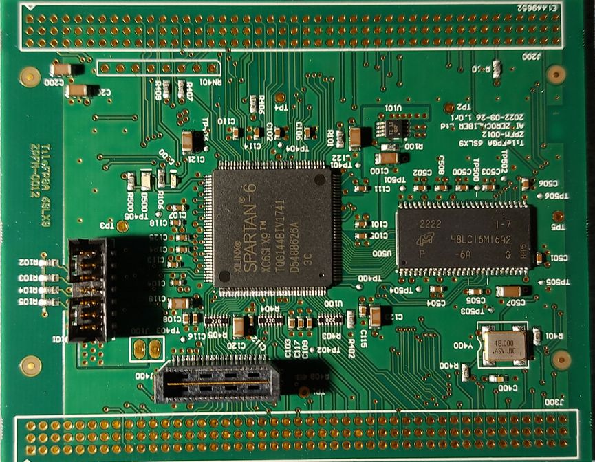
As FPGAs are also hit by the component shortages in the semiconductor market, the design was based on AMD/Xilinx Spartan 6LX9 device, as this was in stock. The fact that the device is in a QFP package (as opposed to BGA) allows a less expensive PCB design with easier debugging, as all pins can be probed.
TileFPGA Board
The board was designed in less than 2 weeks and it came into our lab for verification. In order to test the board, we must connect it to our TileMCU through a backplane, and run the appropriate firmware that will load a valid configuration to the chip. A suitable test design with proper pin constraints was created.
After the assembly of the missing parts, the TileCUBE assembled with the microcontroller and the FPGA.
TileFPGA in Unconfigured State
The initial power-up lit our default LEDs (orange LED lit, means that the FPGA is unconfigured). We had to compile a test design with the updated pin-out from the Perseus CFE board to the TileFPGA. The design was placed at the SDCard. The firmware was adjusted to load this FPGA bitstream, so we can test the MCU and SDRAM interfaces.
FPGA in Configured State
After the FPGA was configured, we tested the Mini-FlexBus interface. We used the debugger to inspect the register area and confirmed the visibility (read operations). Registers were also written to verify that the interface is working as expected. We tested the LED state change (green color seen in the above photo) by changing the relevant bit in a register.
The next phase was to test the internal Block-RAMs. Initially the internal logic did not route the memories to the FlexBus interface (this was a design feature). the values seen in the memory space are 0xFFFF (due to the pull-ups inside the FPGA logic).
Block-RAM Access Enable and Test
Setting the respective enable bit in the control register the memory space can be written and the values are retained. Note that the default memory values seen by the Bus are 0xFFFF, but as soon as we step an instruction after the memory enable bit is set, the debugger refreshes the memory contents that are now zero.
These tests concluded the basic Mini-FlexBus interface and the internal Block-RAM interfaces. In the next post, we will test the SDRAM.
The TileMCU Coldfire version completed its first set of tests, completing the integration of the USB stack from Freescale/NXP to the RTOS.
Using POSIX-style drivers (or any standard way of interfacing) we were able to replace the Serial input of the Command Line Interpreter (CLI) with the USB one.
The code change was a very simple one, replacing just the name of the driver.
Code Excerpt of Selectable Driver
So essentially we define a preprocessor macro with the name of the required driver. As both the USB-CDC and the Serial driver have the same API, they can be interchanged at will.
Here we do this on compile time. Another option would be to mirror both interfaces and have at the same time either USB or Serial I/O. For now, we decided to keep it simple as we have to test the rest of the boards to complete our hydrophone system.
USB Enumeration
At first, the USB enumeration was checked to see if the basics worked. Then we opened with our terminal the respective virtual serial port and start testing the CLI.
CLI Test Example
The CLI was tested to ensure that there were no problems using it and testing some other functions like the SD Card mounting and FAT access.
As we have completed the first phase of testing we can move on to the next boards for testing. We will return back to this board to test the Mini-FlexBus interface with the FPGA.
The concept of a flexible and scalable system is a usual requirement for many applications. We initially started this flexibility by integrating MCUs with FPGAs on the same board. These created the initial Perseus Family Platform boards that we used for the development of applications.
Later on, during the MARI-Sense project, it was evident that the form factor should be more compact while features should be more selectable. In that spirit, we created the TileCubeTM System. Toward implementation of the platform, we designed boards for a complete hydrophone system, including microcontroller boards, FPGAs, and analog front-ends.
Due to component shortages, we were forced to design and use existing parts that we had in stock for the boards. Some boards are already designed with higher-performance microcontrollers waiting to have the new parts in hand. The flexibility of the system allows using different MCU boards in a backward-compatible manner.
The first board of the Tile System is the microcontroller. This version is based on Coldfire MCF52258.
CAD Model of TileMCU_CF
Soon the boards arrived to our lab and we started the board bring-up process and testing.
Actual TileMCU_CF Sample
We confirmed the firmware configuration changes to support the new I/O assignment and installed COFILOS to test the system. Soon we had a system working with serial communications, command line interface (CLI), etc.
First Light (Blinking) of Firmware
Next steps were to verify the SDCard interface and we tried the first time the Digilent Digital Discovery tool for capturing SPI data.
SDCard SPI Checks
Finally, we confirmed the proper operation of the SDCard and through the CLI we sneaked into the first sector of the device.
SDCard First Sector
Initially, the same board was designed with another microcontroller in mind, but due to component shortages, we had to re-spin the board with Coldfire. It was a fast race to quickly redesign the board, build it and make it work, within our deadlines. This gave us the motivation to complete the rest of the boards with the same speed, so we can see the full system ready and explore the potential of the system.
If you are interested in this platform feel free to contact us.
In the past 18 years I have been using a 100MHz two channel oscilloscope TDS3012B from Tektronix, which was using the new at the time Digital Phosphor technology (DPO). With a bandwidth of 100MHz back then it was sufficient for embedded design and debugging. I was missing the serial decode capabilities, but I was able to program a Python script for this purpose. For more information see my article in CodeProject.
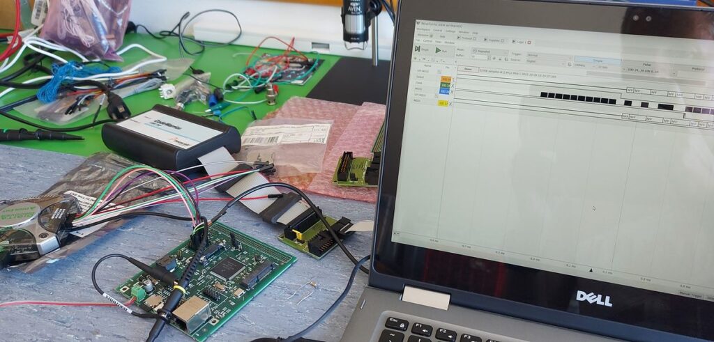
Debugging a system with Atmel AVR and Xilinx Spartan (5K gates) device
Back then it served me very well, although in some cases I would like to have four channels to help me resolve some problems. Not a showstopper anyway, I have been used to have less than ideal equipment. Recently the ethernet interface failed and this reduced the capabilities of my old instrument. In addition, my newer embedded boards started using SDRAMs or HDMI and the signal bandwidth of the scope was below my debugging needs. I had to guess the clock phase on my FPGA-SDRAM interface looking to sinewaves on my scope and trying an educated guess for the correct PLL phase delay. Fortunately, the first guess for the phase difference was correct, so this went smooth and my SDRAM worked fine without much hassle. The old floppy also prohibited data transfers or firmware updates.
According to Altium Designer research about new PCB designs, the trend is to go to boards with 500MHz. Although this might seem a little high for microcontrollers, I started feeling the pressure to go above 100MHz and for some newer serial protocols even higher. I had a SDRAM 133MHZ, but DDR starts to be more mainstream even for embedded systems. Purchasing a scope is an investment for the next 10 years and hence the capabilities should match at a great extent the future requirements. If we go to platform FPGA boards, like Ultra96 or PynQ, there are serial interfaces that can achieve clock frequencies above the 100MHz limit. So, I thought that my next scope should be certainly at the range of 350MHz. So, I decided to move on to a new scope like the MSO44 from Tektronix. A big thanks to Vector Technologies which helped me with my decision. In the next paragraphs, I will present some of the features from my preliminary tests of the new instrument. I still keep my TDS3012B around, as a secondary instrument for field work.
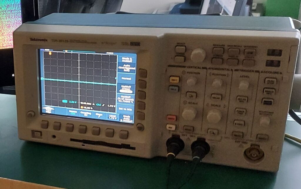
Last days of my TDS3012B Sitting on my lab, while expecting the MSO44.
Thank you TDS3012B for your service all these years!!
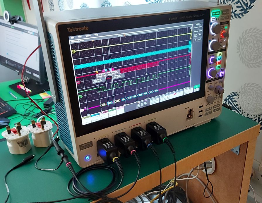
MSO44
The new instrument has four analog channels. This alone is an important upgrade. I can check full SPI bus with enables and clocks or combination of analog and digital lines on my board. A rarely used more than 4 channels unless I had to deal with a digital parallel bus. Even then looking at some control signals and one of the data could give you an idea of the situation. Nevertheless, an analog probe can be replaced by a digital counterpart with 8-channels digital inputs and used as a logic analyzer. You lose one analog channel for this, but it is a reasonable compromise. Other vendors provide this functionality without the analog probe loss, but I do not believe or remember a case in the past that this would be an issue.
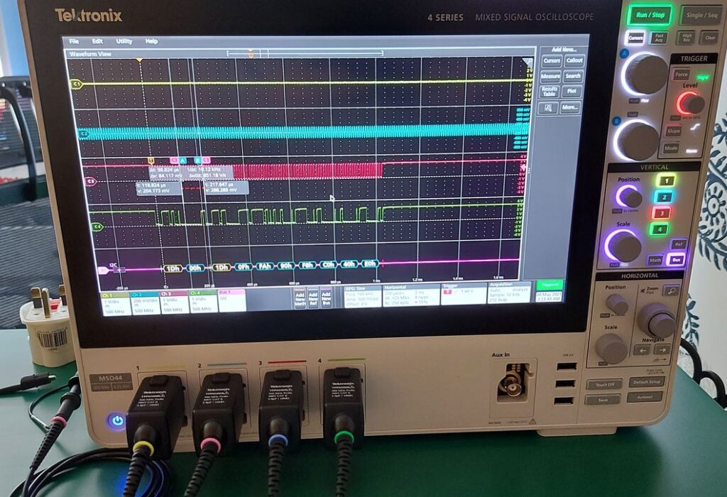
A quick view of the MSO44 in action
The next major upgrade is the bandwidth of 500MHz. Hey, I can check my SDRAM clock easily now… I want to check at some point my HDMI signals (at 250MHz). The 500MHz though can be used also for RF applications at 433MHz, through the spectrum analyzer feature. Really neat.
The arbitrary function generator feature is really useful as with one instrument I can also exercise my circuits. I plan to use this feature for testing the Hydrophone Analog Front End and the FPGA data capture.
I am not going to stay at the UI features most instruments in this category have recently, the large touchscreen etc. Having a large screen estate is important to view multiple signals.
One important aspect of the new generation of instruments is that they offer upgrades by license. So, you can upgrade the bandwidth or some features (more serial busses decoding etc) by purchasing them later according to your needs or projects. This provides a more viable solution where you start with some specific requirements and you can scale up the instrument according to your needs later-on.
Serial Decode
The instrument supports serial decoding of common protocols like RS232, I2C or SPI. This is useful for debugging peripherals or components to your microcontroller. To test this feature I tried an I2C interface on one of my boards. The abundance of screen area is useful to put all the signals without too much clutter and in addition have the serial bus decoding.
Serial Bus decode of an I2C bus
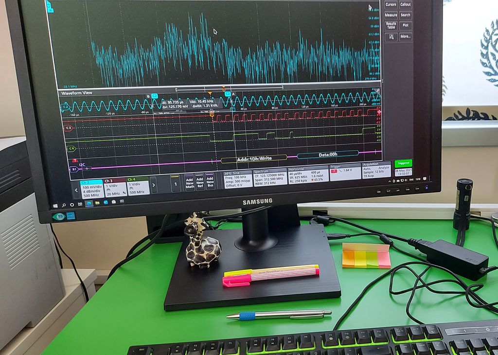
Web Interface
Connectivity is important, so the instrument comes with a bunch of USB ports and an ethernet port for network. This is what I used with a web browser to mirror my MSO screen to my desktop PC. Extremely helpful if you want to control the instrument from the same place as you control your debugger. No need to turn your chair around to turn knobs.
MSO screen view on my desktop PC
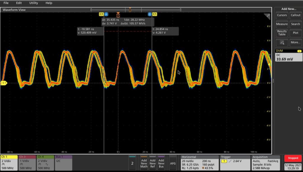
Jitter Tests
On one of my boards, I knew that there is some jitter on my clock. So, I decided to test the DPO capabilities and look in more detail on this signal. I can see the probability of states clearly. I want to delve more on this feature in the future.
Clock Jitter seen through DPO
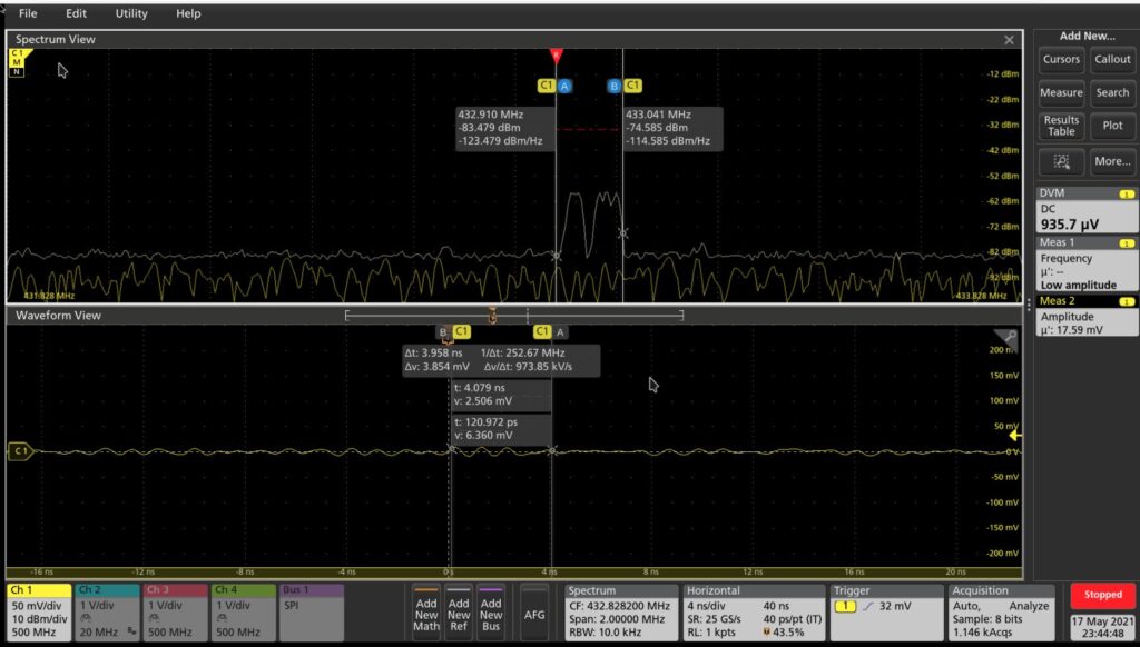
Spectrum Analyzer
Yes, many engineers would say that this is the FFT button or feature found on most of the scopes, so what’s the big deal. Well, nope. The FFT feature exists in the math menu and is not the same with the spectrum analyzer feature, which works like a spectrum analyzer. I mean you need to setup video bandwidth, resolution bandwidth and so on, as you would do in an actual spectrum analyzer. In addition, changing the time domain signal (scaling-resolution) does not affect the spectrum and vice-versa. I read about this feature on the website when looking at the specifications and I was keen to see it in action. Having worked with spectrum analyzers in the past, I got pretty familiar with the parameters. This feature exists inside the channel settings (tap on your channel and select spectrum tab). Testing this feature, I tried a remote of 433MHz. The probe was attached at the antenna signal on the receiver side.
Spectrum of a remote at 433MHz
I even went further. I have some LoRa devices working at 433MHz and wanted to confirm that this is their center frequency. As LoRa uses broadband transmission, I set-up my instrument to capture and hold the maximum level. So after a while transmitting, the spectrum started to show activity, by filling bands.
Spectrum max hold at 433MHz, LoRa transmission
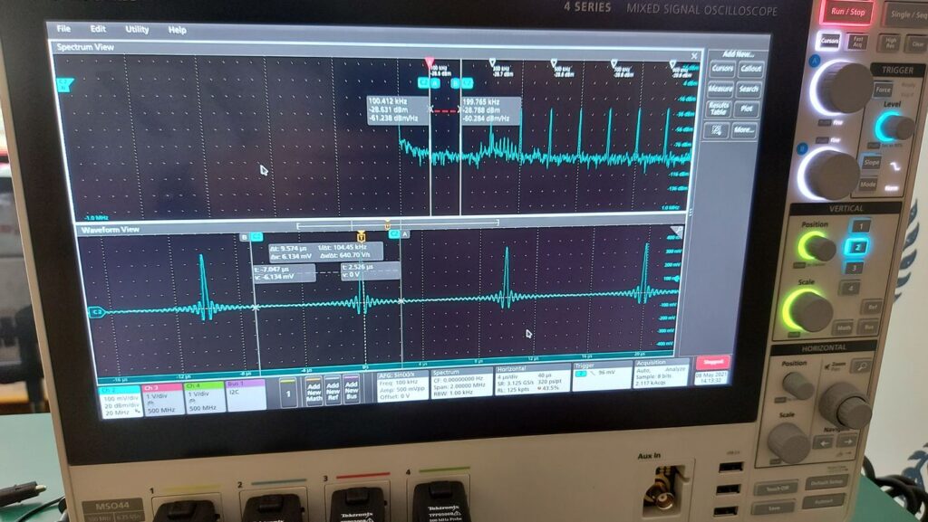
Arbitrary Function Generator
Providing stimulus to your circuits is essential when designing and testing analog to digital converters. Applying some basic stimulus may help you check design elements and ensure that the basics work. For more thorough testing you will need a dedicated instrument. In this case the arbitrary function generator is used for the first line of defense. Here a sinc function is output and its spectrum is displayed.
Arbitrary Function Generator and Spectrum
Conclusion
I will need to spend lots of time to test every aspect of the new instrument. I am already using it in my projects, and I am getting used to it. Albeit the complexity of the functions, I can navigate around, put the right settings without hassle, giving me time and insight and let me be productive. I have a long queue of things that needs development and testing that this instrument will help me a lot.
Our laboratory is now massively upgraded and ready to win the next battles!
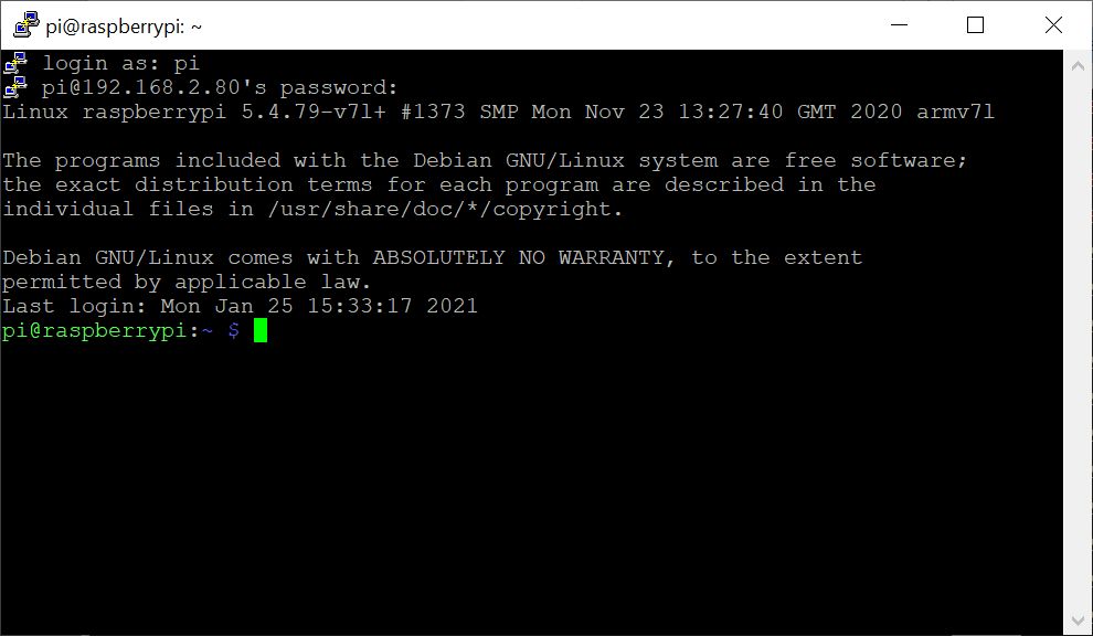
It is assumed that you have already setup the Raspberry Pi to have remote desktop and SSH agents active. I also have setup my network to assign a specific IP to this device both for wired or wireless operation. It is also assumed that you already installed git or any other tools you require for development. We used the default Raspbian Linux. Login in with SSH should present something similar as the next picture. Of course, you may use a remote desktop environment; select which best fits your taste.
Raspberry Pi Login Screen
Notice that this is a Linux 5 kernel. This is important mostly for driver’s compatibility or support with the DAC+ADC Pro board. However, we did not face any real issues with our setup.
Python can get messy with packages and proper system configurations. Note that the Raspberry Pi image comes with both Python2 and Python3 interpreters. Writing simple python runs the 2.7 version while running python3 calls the Python 3.x interpreter. Keep this in mind.
In our case, we used the Python3 setup. First, we created a virtual environment to install packages. There are many ways to do the setup. You may try the anaconda system (although the link below for TensorFlow says that this will not work), which will take care of any dependencies and install all the packages, or you can follow on here and see the more tedious manual approach. The idea is to have a system set up in our Raspberry that matches the one we use in our desktop environments to ensure maximum compatibility and help us with testing.
Download the virtualenv package:
$ sudo pip3 install virtualenv
Then we can select a directory to do our development and create the virtual environment there:
 $ cd UnderwaterSoundProcessing
 $ virtualenv audioml
 $ cd audioml
 $ source bin/activate
 … do something…
 $ Deactivate
If you check the requirements.txt in the github repo, you will notice a long list of items that must be installed along with their version numbers. If you try the simple command:
$ pip3 install -r requirements.txt
You will fail miserably. The reason is simple. Kapre requires TensorFlow version at least 1.15, but default TensorFlow for Raspberry is 1.14.
TensorFlow 2 cannot be installed by default on RPB Pi4. We followed the instructions from this link:
The script used is on a google drive (check contents, security and stability issue)
TFLite can provide significant improvements in prediction. You may convert your normal models to Tflite for faster processing. Need to test on each application if accuracy is maintained.
When installing in venv do not use sudo. In case you did (as I did), reinstall (last step) tensorflow without the sudo. Test that Tensorflow is installed from python before continuing.
If in python interpreter you are able to import the tensorflow package as stated in the link you are good to go.
For Tensorlow and Numpy packages we install the ATLAS library.
$ sudo apt install libatlas-base-dev
Another issue we faced was the LLVM library. Numba 0.48 requires v7 of LLVM and not v9.
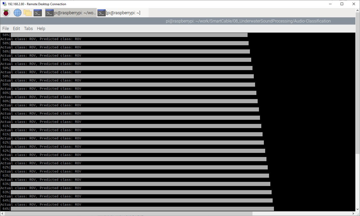
We run our predict module to see it working. We had already trained previously on a desktop PC the machine learning network to classify a mixture of sea sounds taken in a previous experiment and from the web.
$ python predict.py
Running Training on Raspberry Pi
All these are nice, but still where is the hydrophone? Next steps describe the process to properly interface the DAC+ADC Pro module.
Although the kernel is 5, we needn’t to do the work-around presented for the EEPROM. First, we tested the playback. Please note that the device is not the default, but rather the sysdefault as seen after the next command.
Sound Devices List
The following commands will output sound from the left and right channel respectively.
The values of this command are steps between 0 and 104 and will set ADC volume 0.5db/step. So 96 is about 48dB. You may adjust this value to a lower level depending on the sensitivity. A 33dB gain should work just fine. You may retry to record again and observe the VU meter levels.
For python to access the audio device, we installed the ALSA audio:
To ensure that the same exact code is used either for off-line prediction and on-line prediction, we used a file wrapper in python. The sampling function performs a sampling for a duration (like 1 second) and stores the result in a file. Then the main loop acquires this file and processes it like it does off-line content.
def readdaq(self):
     loops = int(self.sample_dur_seconds * round( (self.fs_Hz / self.chunk) ) )
     frames = []
     sample = np.array(frames)
     while loops > 0:
         loops -= 1
         # Read data from device
         l, data = self.inp.read()
         if l>0:
             if l!= self.chunk:
                 print("Sampling Error ", l)
             frames.append(data)

     wf = wave.open('/mnt/tmpfs/sample.wav', 'wb')
     wf.setnchannels(self.channels)
     wf.setsampwidth(2)
     wf.setframerate(self.fs_Hz)
     wf.writeframes(b''.join(frames))
     wf.close()

     batch = self.readfile('/mnt/tmpfs/sample.wav')

     return batch
Note that the file is saved on a temporary location. This is a ram drive created as follows:
The reason of using a ram drive is that we do not want to wear out our SDcard, or have slow-downs due to file system activity. We use this scratchpad area to write the samples and use them for processing. Then the sample is overwritten by the next sample.
This way we streamline the testing process and are able to run the same code with or without hydrophone, either on desktop, or on Raspberry Pi.
Conclusion
Using open-source software and off-the-shelf hardware we are able to have a platform for sound classification using machine learning. We created a uniform testbed that can be used to test either on-line or off-line the methods employed for evaluation purposes.
Acknowledgment
The SMART Cable was developed through the SMART Cable Project. This project is part of the Research & Innovation Foundation Framework Programme RESTART 2016-2020 for Research, Technological Development and Innovation and co-funded by the Republic of Cyprus and the European Regional Development Fund with grant number ENTERPRISES/0916/0066.
This project is also part of the MARI-Sense Project INTEGRATED/0918/0032. The MARI-Sense project develops intelligent systems that allow human operators to make sense of the complex maritime environment for applications including transport and shipping, coastal tourism, search and rescue, and maritime spatial planning.
In scientific projects, it is often needed to sample sounds from remote locations, for classification or other purposes. As data link rates may be low or unreliable, transmitting raw samples to inland processing centers may not be an option. An alternative is to do off-line processing in batches. This means that raw data are stored in non-volatile memory untill a physical visit replaces the memory media and uses the first batch for processing after any events occurred. It is obvious that a module that performs real-time classification will have to send a very small amount of data to, possibly cloud-based data centers.
Towards this direction, we will show how to build the basic elements needed for such systems using simple parts and open-source software packages, to provide a platform to build classification systems for hydrophone sensors.
Hardware
The hardware we are going to use for this example is based on Raspberry Pi 4.
Raspberry Pi module
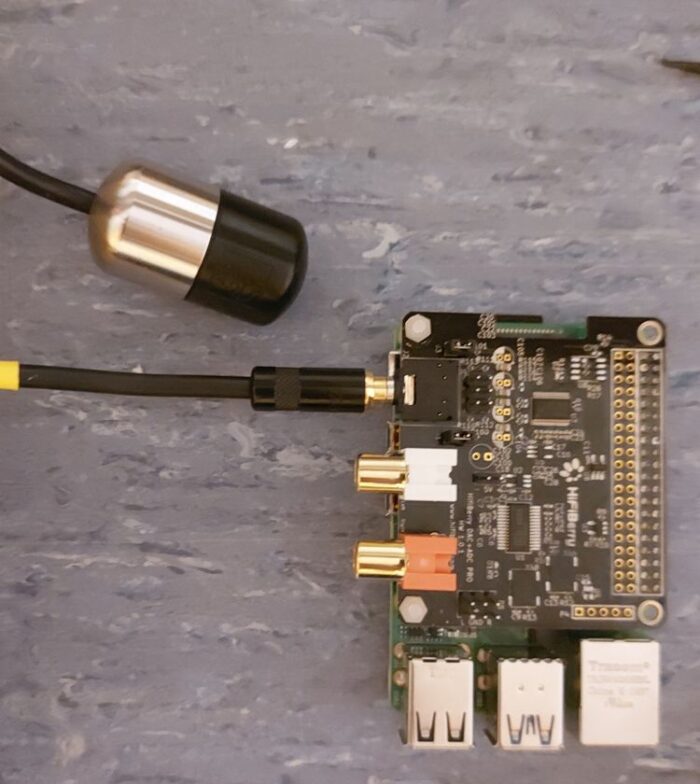
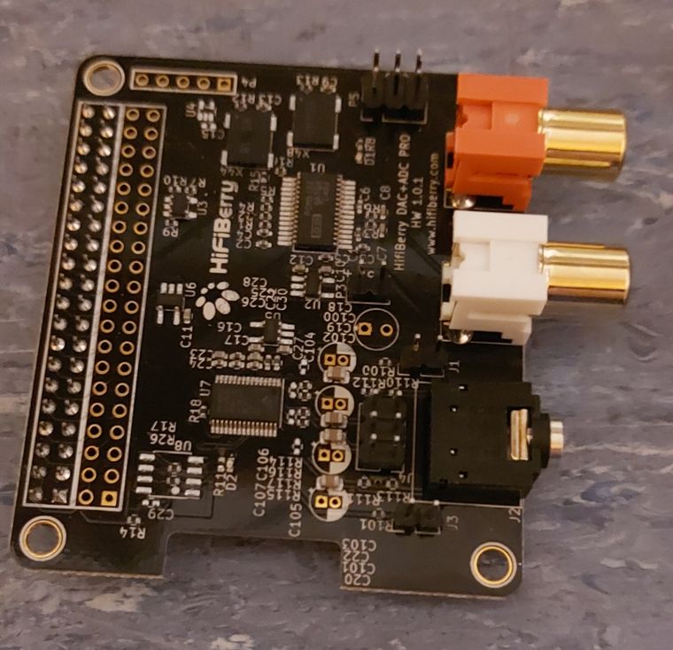
To interface we use a hydrophone an analog to-digital converter is needed. For our experiments we used the DAC+ADC Pro from HiFiBerry (HiFiBerry DAC+ ADC Pro | HiFiBerry). This module offers both audio input and output. In our case, we are only interested for the audio.
HiFiBerry DAC+ ADC Pro
This HAT is placed on top of the Raspberry PI. To mount properly the module, we used the following items as seen in the next picture.
ADC and Raspberry Pi side to side
We used two of the nylon stands to hold the front side of the HAT. We skipped the back nylon stands as they wouldn’t allow to fully insert the connector. In the picture above we have assembled the front stands in the Raspberry Pi 4 and we are ready to connect the HAT. Also note the small nylon bolts for securing the HAT and two jumpers we will need for the hydrophone.
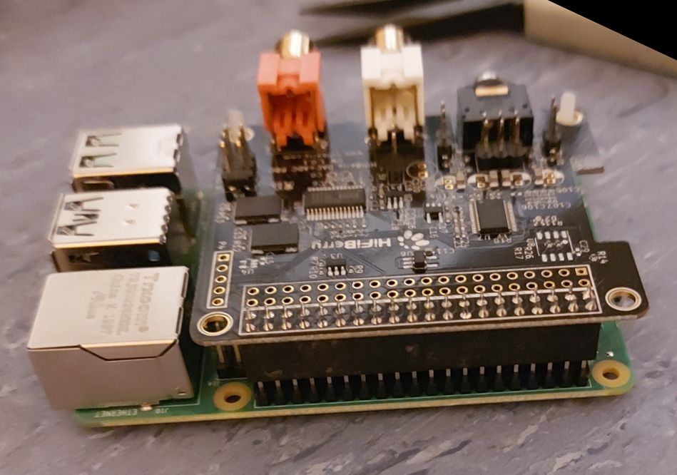
Next, we connect the HAT on top of the Raspberry PI module. We fully insert the connector; we should not see any naked pins protruding from the bottom as seen in the picture.
ADC on top of Raspberry Pi
We then place the bolts to be ready for tightening the HAT. The HAT will have a slight inclination as the front stands will keep it slightly upwards, in respect with the fully inserted connector.
ADC front side mount
After completing the mechanical fit, comes the jumper settings. The two jumpers J1 and J3 must be placed to provide power to the hydrophone. This is because our hydrophones are behaving like condenser microphones and they do not generate their own voltage. Make sure you check which type of hydrophone you use as depending of the hydrophone technology you may not need this power; Failing to properly identify the type of hydrophone may damage either your equipment.
ADC Jumper Settings
Our hydrophone is the H2a Aquarian Audio from Aquarian Hydrophones. Next pictures show the hydrophone and its connector ready to be connected on the platform. H2a Hydrophone (aquarianaudio.com)
H2a Hydrophone Just Before Connection
Next, we connect the hydrophone to the 3.5mm Jack input of the DAC+ADC Pro HAT and we are ready to go from the hardware standpoint.
H2a Hydrophone Connected
Conclusion
This ends the first part of the smart Hydrophone, concluding the Hardware. A setup showing how to integrate off the shelf components to support Hydrophone sound sampling from the sea was presented.
Acknowledgement
The SMART Cable was developed through the SMART Cable Project. This project is part of the Research & Innovation Foundation Framework Programme RESTART 2016-2020 for Research, Technological Development and Innovation and co-funded by the Republic of Cyprus and the European Regional Development Fund with grant number ENTERPRISES/0916/0066.
This project is also part of the MARI-Sense Project INTEGRATED/0918/0032. The MARI-Sense project develops intelligent systems that allow human operators to make sense of the complex maritime environment for applications including transport and shipping, coastal tourism, search and rescue, and maritime spatial planning.